Note

This page was generated from a Jupyter notebook. Download: pole_figure.ipynb

Pole figure notebook example

from matplotlib.colors import LogNorm
import numpy as np

import cdiutils

cdiutils.plot.update_plot_params()

Path to the data that contains the orhtogonalised Bragg peak, along with the corresponding grid of q values.

If you have run the BcdiPipeline.preprocess() function, you can find the data in the results folder, in the "S<scan>_preprocessed_data.cxi" file.

path = ("path/to/data.cxi")

Load and plot the data

with cdiutils.CXIFile(path, "r") as cxi:
    data = cxi["entry_1/data_2/data"]
    qx = cxi["entry_1/result_2/qx_xu"]
    qy = cxi["entry_1/result_2/qy_xu"]
    qz = cxi["entry_1/result_2/qz_xu"]
    shift = cxi["entry_1/result_2/q_space_shift"]

print(qx.shape, qy.shape, qz.shape, data.shape)
voxel_size = (
    np.diff(qx).mean(),
    np.diff(qy).mean(),
    np.diff(qz).mean()
)

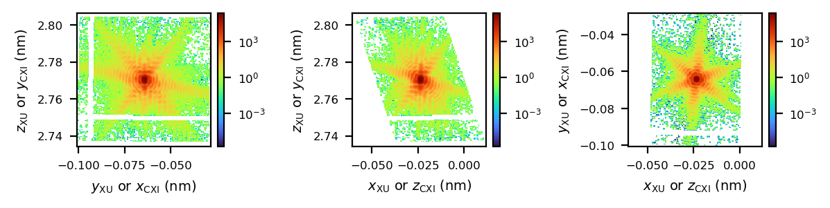
fig, axes = cdiutils.plot.plot_volume_slices(
    data, voxel_size=voxel_size, data_centre=shift,
    norm=LogNorm(), convention="xu", show=False
)

cdiutils.plot.add_labels(axes, convention="xu")
fig

(141,) (146,) (146,) (141, 146, 146)

Usage of cdiutils.analysis.pole_figure

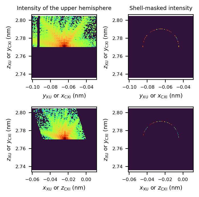
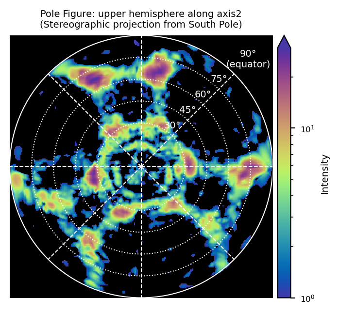
The cdiutils.analysis.pole_figure function generates a crystallographic pole figure using stereographic projection. This method maps 3D diffraction intensity data onto a 2D plane, providing a visual representation of the crystallographic orientation distribution.

Parameters:

• intensity (np.ndarray): A 3D array of intensity values representing the diffraction data.

• grid (list): A list of 1D arrays defining the orthogonal grid (e.g., [x_coords, y_coords, z_coords]).

• axis (str, optional): Specifies the projection axis and hemisphere:

  • "0", "1", "2": Upper hemisphere projection onto the equatorial plane.

  • "-0", "-1", "-2": Lower hemisphere projection onto the equatorial plane.

  • The absolute value of the axis determines the normal plane:

    • |axis|=0: Project onto the yz-plane (normal to x-axis).

    • |axis|=1: Project onto the xz-plane (normal to y-axis).

    • |axis|=2: Project onto the xy-plane (normal to z-axis).

  • Defaults to "2" (upper hemisphere projection onto the xy-plane).

• radius (float, optional): Radius of the spherical shell for data selection. Defaults to None (0.25 * max radial distance).

• dr (float, optional): Thickness of the spherical shell. Defaults to None (0.01 * radius).

• resolution (int, optional): Resolution of the output 2D grid (number of points per dimension). Defaults to 250.

• figsize (tuple, optional): Size of the output figure. Defaults to (4, 4).

• title (str, optional): Title for the plot. Defaults to None.

• verbose (bool, optional): If True, prints and plots additional information. Defaults to False.

• save (str, optional): File path to save the plot. Defaults to None.

• plot_params (dict, optional): Additional parameters for the plotting function.

Returns:

• tuple:

  • (grid_x, grid_y, projected_intensity): The 2D grid coordinates and intensity values.

  • (fig, ax): The figure and axis objects for the plot.

# Basic usage with default parameters
(grid_x, grid_y, projected_int), (fig, ax) = cdiutils.analysis.pole_figure(
    data,
    [qx, qy, qz],
    radius=0.020,
    dr=0.0002,
    axis="2",
    norm=LogNorm(1, ),
    verbose=True,
)

Projection axis: 2, selecting upper hemisphere with observer at South Pole
Selected radius: 0.020 and spherical shell thickness: 0.00020